What's New in FactSage 7.0

(October 2015)

The FactSage 7.0 Update/Installation program permits you to upgrade/refresh any version of FactSage to FactSage 7.0. You can also install FactSage 7.0 directly on to a new PC.

With the new additions and extensive modifications FactSage 7.0 is a major update to the FactSage package. The total number of files is now over 12,000 (was 7,000). The major version number has been changed from 6 to 7 because the solution database structure has been completely rewritten. Old solution *soln.sda files in 6.4 will no longer be accessible - they have been replaced by the new *soln.sln and *soln.sdc formatted databases. The modules that access the solution databases (View Data, Equilib, Phase Diagram) have been programmed to access the new solution database structure.

What follows is a list of the more important programming, database and documentation changes in FactSage 7.0 (2015) with respect to FactSage 6.4 (May 2013).

1. General:

2. Modules: 3. Databases:

1. General:

  • FactSage 7.0 News
  • FactSage 7.0 Update/Installation/Menu
    • Download FactSage 7.0 - The FactSage 7.0 Update/Installation program contains the complete 7.0 package of software, databases and documentation. It can be downloaded from the Internet. For details visit www.factsage.com and click on 'Download Service' and then 'FactSage 7.0 Update/Installation '. For certain installations it may not be possible to download the file - for example you may get an error message such as 'webpage cannot be found'. This could be because the security settings on your computer are blocking the transfer of a ".zip" file or the file is too large to be downloaded. Check with your IT group.

    • FactSage Installation The FactSage 7.0 Update/Installation program is a one-stage installation and update program. The program runs a self extractor that automatically performs the extraction operation before starting the installation. Although you can update an earlier version of FactSage that is already installed on the PC (FactSage 6.0, 6.1 ...) we recommend that you install FactSage 7.0 in a new location on the PC. See below (Update/Refresh FactSage 7.0) for more details.

    • Server/Client Installation - For a client installation on the network, the program FactSageClient enables the Client workstation to locate the Server installation. The program is run prior to the FactSage 7.0 setup program and is well-suited for Windows 7, Windows 8 and Windows 10 installations. Details are given in ShowMe which is part of the installation package.

    • Server/Client Update - If the FactSage Client is already running FactSage on a network installation and the Server installation is then updated (for example a new version or new databases), the Client installation will not be updated until a new day. This default action can be overridden - to immediately update FactSage on the Client workstation, in the FactSage Main Menu of the client PC click on 'Tools > FactSage Network > Refresh Client installation ...'.

    • Windows Vista, Windows 7, Windows 8, Windows 10 - FactSage 7.0 has been successfully installed and tested under Windows Vista, Windows 7, 8 and 10 operating systems. All programs run as designed including the Solution module (see below). The dongle drivers distributed with FactSage 6.4 (or earlier) are outdated. The latest drivers (see below) are very well suited for installing under Windows 7, Windows 8 and Windows 10.

    • Windows XP no longer supported by Microsoft - FactSage should still run under Windows XP even though Windows XP is no longer supported by Microsoft. According to Microsoft if you continue to use Windows XP now that support has ended, your computer will still work but it might become more vulnerable to security risks and viruses.

    • Sentinel HASP Drivers - FactSage MemoHASP dongles are also referred to as Sentinel Security Keys and more recently Sentinel LDK keys. The dongles are now supplied by SafeNet Inc. In FactSage 6.4 (and earlier) it was often difficult to install the drivers especially under Windows 7, Windows 8 and Windows 10. FactSage 7.0 employs new installation software from SafeNet Inc. and it is now fairly straight forward to install the drivers. For instructions click on 'Tools > Sentinel Security Key > Information ...'

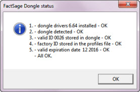
    • FactSage dongle status - When a valid HASP dongle is attached to a USB port on the computer you are able to run a standalone version of FactSage. If FactSage issues an error message about a 'missing or invalid FactSage HASP security key' it goes into the FactSage SetUp mode with a green screen. There are several factors that can cause this to happen.

      There is a new feature in FactSage 7.0 which displays the status of the FactSage dongle attached to the computer. This helps you to diagnose the source of the error message.

      • Run FactSage 7.0 and display the FactSage Main Menu Window.

      • Click on 'Tools > FactSage dongle status > Explanation of dongle status... ' and follow the instructions.

      The 'FactSage dongle status' Window shown here is for an installation where a valid FactSage dongle is attached and everything is in order (i.e. 1 - 5. All OK).

  • Update/Refresh FactSage 7.0

    The FactSage 7.0 Installation program enables you to update/refresh FactSage 7.0 software, documentation and databases to the full FactSage 7.0 package.

    You can update/refresh a FactSage Standalone computer or a Network Server. In the case of a network installation it is only necessary to update/refresh the Network Server.


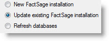
      IMPORTANT: Please read before selecting the option 'Update existing FactSage installation'.

      If you select this 'Update' option to overwrite a FactSage 6.4 (or earlier) installation with the software and databases of FactSage 7.0, this may lead to unintended consequences:

      • If you have a permanent licence to FactSage and have paid for updates of some but not all of your databases (for example: you have updated the FACT solutions databases package but not FSstel), then the databases that you have not updated will not be accessible in FactSage 7.0 and will be deleted. (For example: FSstel would be deleted from the \FACTDATA folder).

      • Private solution databases (*soln.sda files) that we have prepared for you in the past will not be accessible in FactSage 7.0 and will be deleted from the \FACTDATA folder. Such databases need to be converted to the new solution format (*soln.sdc files) - contact your database provider for details.

      • Some of your previous calculations may give slightly different outputs when you use the updated databases. Also in some cases solution phases have been removed or renamed and new ones added.

      • Some databases (SGTE(2004), FSlite, FSnobl, SGSL) have been discontinued in FactSage 7.0. These databases will be deleted from the \FACTDATA folder.

      To avoid these consequences, we recommend that you keep your current FactSage 6.4 installation and select 'New Factsage installation' and install FactSage 7.0 in a new folder (directory).


  • General
    • Slide Shows on FactSage Applications
      - called from 'General > Slide Shows > FactSage Applications ...'.

    • Ferrous Processing Slide Shows

      Almost 200 new slides have been added to the ferrous presentations to bring the total to over 400 slides. The single presentation has been split into 5 new slide shows :

      • 1. Ferrous Processing: Review of Engineering Thermodynamics
        - including Gibbs energy equations, Gibbs energy minimization, Ellingham diagrams, solution thermodynamics, Gibbs Energy vs. Phase Diagram, thermodynamic database development, dilute solutions, standard states, etc.
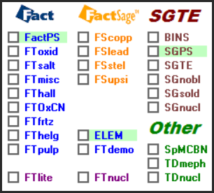
      • 2. Ferrous Processing: Database Selection
        - how to select the databases (FactPS, FToxid, FTmisc, FSstel) and their phases (gaseous species, stoichiometric solid and liquid species, slag, spinel, monoxide, olivine, etc. solutions) in the various steelmaking calculations.
      • 3. Ferrous Processing: Applications I
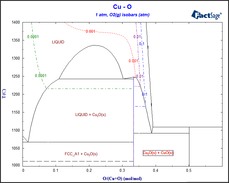
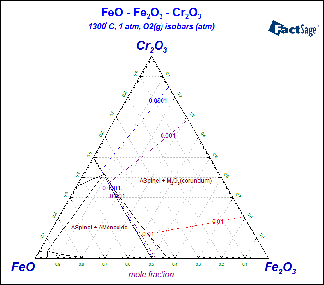
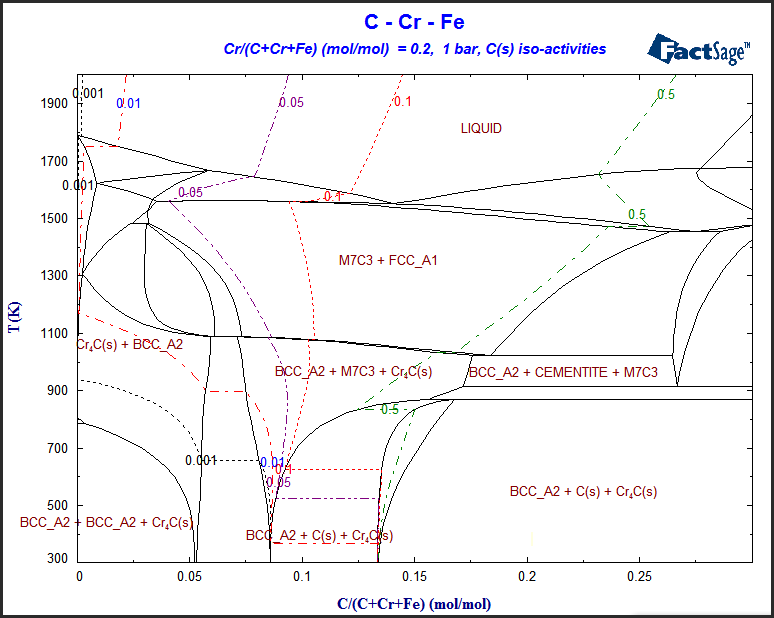
        - simple transition calculation; formation, precipitate and composition targets; streams; vacuum degassing activity calculations in binary system; ternary iso-activity line calculation; CaO-SiO2, CaO-Al2O3-SiO2, Fe-Cr-O2, CaO-FeO-SiO2-5%MgO at Fe saturation, etc. phase diagrams; refractory/slag interactions; Paraequilibrium for A3 temperature of Fe-C system / Rapid quenching; Si steel desig; etc.
      • 4. Ferrous Processing: Applications II
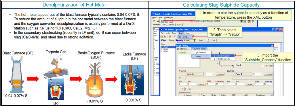
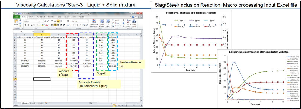
        - Slag liquidus temperature depression; Dissolution mechanism of inclusions into molten slag; Non-metallic inclusion formation: oxide metallurgy; Inclusion control in Mn/Si killed steel; Refractory dissolution in molten slag (RH degasser); Ladle glaze formation; V2O3 addition to liquid slag (Henrian solution: optimization of parameter); Carburization and de-carburization of steel; Viscosity of slags: Einstein-Roscoe equation for semi-liquid state; etc.
      • 5. Ferrous Processing: Process Simulation
        - macro processing of secondary steelmaking, simplified BOF process, slag/steel/inclusions interactions.

      Sample screenshots of new slides in the Ferrous Processing Slide Shows

  • Documentation
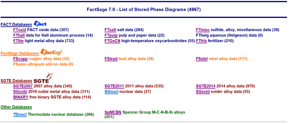
    • The 'list of stored phase diagrams' posted in the FactSage Browser has been updated to 4967 (was 3460). SGTE2014 and SpMCBN are new in FactSage 7.0 - see 3. Databases for details.


    2. Modules:

  • New Solution Database Format

  • Solution
      In FactSage 6.4 and earlier versions it was not possible to run the Solution program under Windows Vista, Windows 7 and Windows 8.

      This problem has been resolved and it is no longer an issue.

      The above message no longer appears in FactSage.

      The Solution module has been completely rewritten and replaces the old module that was programmed over a decade ago.

      Old private text data *.dat files (e.g. Solution.dat, ExamSoln.dat) and old private binary data *.sdb files (e.g. UserSoln.sdb, PrivSoln.sdb) are still accessible in FactSage calculations (View Data, Equilib, Phase Diagram) but cannot be directly edited in the Solution module. However, old data may be imported by the Solution module into the new structure and saved as a new private text *soln.sln files (e.g. Copysoln.sln, MyTestsoln.sln).

      Data can be entered and stored using the following solution models: One-sublattice polynomial model (simple, Redlich-Kister or Legendre polynomials, with interpolations to multicomponent systems using Muggianu, Kohler or Toop methods), Compound Energy Formalism with up to 5 sublattices, Two-sublattice polynomial model with or without short-range-ordering, One-sublattice Modified Quasichemical Model, Two-sublattice Modified Quasichemical Model including coupling between first- and second-nearest-neighbor short-range-ordering, Ionic Liquid Model, Unified Interaction Parameter Formalism (corrected Wagner formalism), Pitzer model.

      The Solution module has other new features including :

      • it runs under Windows Vista, Windows 7, 8 and 10.

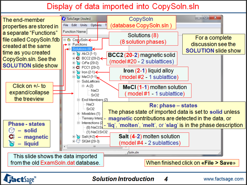
      • expressions of Gibbs energy for solution end-members can be imported from a compound database and stored as functions within the new solution database. The required expressions are selected using the Compound module then imported by drag and drop into the Solution module.

      • the stored functions in a database are accessible to all solution phases within that database.

      • the expanded treeviews of the data provide easy editing access to the 'Functions' and to the solution phase 'Sublattices', 'End Members' and 'Interactions'.
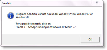
      Details of the Solution module are presented in the new Solution Slide Show (202 pages). See the first pages of the Solution Slide Show for a description of all the models.

      Screenshot from the Solution Slide Show showing data that have been imported
      from the old ExamSoln.dat examples database into the new Copysoln.sln database.
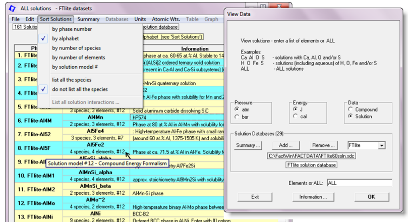

  • View Data

      Solution Dropdown Menu

      Prior to 7.0 it was not possible to list all the phases in a solution database. In FactSage 7.0 the search option for 'all' elements is now included.

      With the new 'Sort Solutions' dropdown menu it is also possible :

      to display all the solutions and sort the phases :

      • by phase number
      • by alphabet (see screenshot below)
      • by number of species
      • by number of elements
      • by solution model #
      with a restriction on the output :

      • list all species
      • do not list all species (see screenshot below)


      Screenshot of the View Data showing the display of all solution phases in the public FTlite database.

      Solution Data

      In FactSage 7.0 it is possible to display the solution data (interactions and expressions) that have been stored in a private database (i.e. soln*.sln file).

      Screenshot of View Data showing the display of solution data that have been stored
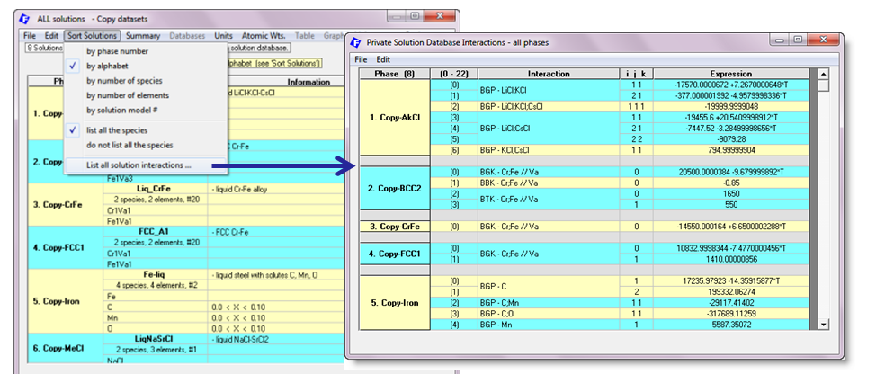
      in the private database Copysoln.sln (data imported from ExamSoln.dat - see above).


  • Predom, EhpH, Equilib and Phase Diagram Modules - limited compound data and gaseous ions (plasmas)

      Limited compound data

      Some solid and liquid compound and aqueous species only have limited data at 25 C - for example the Gibbs energy of formation at 298.15 K is known but not the Cp and enthalpy data.

      In FactSage 6.4 (and earlier) it was possible to include such compounds with limited data in the calculations at 25C. In Predom, EhpH, Equilib and Phase Diagram click on 'Data Search' and check 'limited data compounds (25C)'

      In FactSage 7.0 such species are no longer retrieved when scanning the databases in Predom, EhpH, Equilib and Phase Diagram calculations. This is because these limited data species cause confusion and potential errors when comparing results at different temperatures as they are either being brought into calculation (at 25 C) or dropped from the calculation (when not at 25 C). In most cases the species are unimportant anyway.

      However limited data compounds can still be accessed using the View Data and Reaction modules.

      In FactSage 7.0 the 'limited data compounds (25C)' check box has been removed.

      Gaseous ions (plasmas)

      Gaseous ion concentrations are only significant at high temperatures and only meaningful in plasma calculations. Gaseous ions add a component (the electron) to the calculation and increase the total number of gaseous species. This increases slightly the calculation time because Debye Shielding is also taken into account.

      In FactSage 7.0 calculations are now permitted up to 35 000 K (was 20 000 K). However all the data for Cp are extrapolated from 6 000 K or even lower. For most practical calculations gaseous ions have no effect and so it is safe not to include them in the data search.


  • Equilib

    • Units Window

      Click on the units menu to enter the Units Window you can select either 'Metric SI units' or 'English units'. For example:

        SI units: T(K), P(bar), Energy(J), Mass(mol), Volume(litre)
        English Units: T(F), P(psi), Energy(BTU), Mass(lb), Volume(Ft3)

      In FactSage 7.0 it is now possible to mix the units and select various combination, for example :

        T(F), P(psi), Energy(kwh), Mass(lb), Volume(Ft3)
        T(C), P(psi), Energy(kwh), Mass(lb), Volume(Ft3)
        T(C), P(psi), Energy(kwh), Mass(mol), Volume(Ft3)
        T(K), P(Pa), Energy(J), Mass(lb), Volume(litre)


  • Macro Processing - called from 'Equilib > Reactants Window > File > Macro processing > Run macro ...'

      All the macro files stored in the /MACROS folder have been checked with FactSage 7.0 and the files updated where necessary.

      If you unfamiliar with macro processing go to the Reactants Window, click on 'File > Macro processing > Run macro > Macros Directory ...' and select EquiEx_SET_Variables.mac.

      If you want to see the hidden generated information when you load and run one of your saved Equi*.dat files then select EquiEx_List_Results.mac and specify the Equi*.dat file.

      For an example of how to open and interact (read and write) with an Excel Worksheet (.Xls and .xlsx files) and a Text Spreadsheet then select EquiEx_Xls_Simple_IO.mac.

      For a complete list of examples click on 'File > Macro processing > Macro Processing - Examples ...'.

      1. New Organisation and Documentation

      The Macro Processing program has been reorganised, terminology has been simplified, new commands and functions have been introduced, and new documents have been added.

      Examples of the new commands and functions are given in the macro EquiEx_New_in_7.0.mac.

      The system $Variables have been integrated into $Functions. This has no effect on the macro files.

      Compressed multi-word terminology for commands and functions such as SHELLEXECUTE SHOWLASTPD $FILESHORTDIR etc. have been expanded into SHELL_EXECUTE SHOW_LAST_PD $FILE_SHORT_DIR etc. in order to improve readability. The changes are backward compatible - i.e. the old terminology still works.

      A new document, Macro Processing - Summary, has been added to the menu. This summarizes all the macro variables, functions and commands that are available in macro processing.

      A new document, Macro Processing - Examples, has been added to the menu. This lists the examples and introduces all the Equilib macro files (EquiEx*.mac) that are stored in the Macros folder (typically 'c:\FactSage\Macros\').

      2. New Commands

      2.1 DEBUG

      The new command DEBUG /ON activates the debug mode and displays the DEBUG Macro Window which lists the current values of all user-defined %variables.

      Each time a DEBUG command is issued the DEBUG Macro Window is updated with the current values. It is hoped that this will become a valuable tool in macro processing development.

      As an example, load and run the macro file EquiEx_New_in_7.0.mac that is stored in the Macros folder.

      
      DEBUG /ON        // Activates the DEBUG Macro Window 
      DEBUG /OFF       // Deactivates the debug mode 
                       // - this is the default setting.
      DEBUG 'caption'  // Lists current values of all %VARIABLES 
                       //- 'caption' is the display heading
      DEBUG /DEL %var1 %var2 ... 
                       // Drops %VARIABLES from the debug list
                       // The DEBUG commands are a debugging aid
                       // and have no effect on the macro processing. 


      The screenshot shows the 'DEBUG Macro Window' that is displayed by the macro EquiEx_New_in_7.0.mac.

      2.2 DIM, REDIM

      DIM is new in 7.0 and is identical to VARIABLE. It is now possible to declare a 2-dimensional array using DIM (or VARIABLE).

      If a variable array has are already been declared, it can be re-dimensioned by using the new REDIM.

      
      DIM %A %B(4) %C(2,3) // Declares %A, %B(1) %B(2) %B(3) %B(4),
                           // %C(1,1) %C(1,2) %C(1,3) %C(2,1) %C(2,2) %C(2,3) 
      REDIM %A(0:2,2)      // Re-dimensions %A as %A(0,1) %A(0,2) %A(1,1) %A(1,2) %A(2,1) %A(2,2) 
      

      2.3 Defining tabular values

      
      %total = $E_sMs$  //  total number of product species 
      DIM %mole(%total) %activity(%total) 
          
         // 1. Define the tabular values of activity and moles one at a time
      %1 = 1 TO %total
         %activity(%1) = $E_sa%1$   // or $E_sa(%1)$.  Note () aids in the readability.
         %mole(%1)     = $E_sm%1$   // or $E_sm(%1)$   
      %1 LOOP 
      
         // 2. More efficient way:
      %activity(1:%total) = $E_sa(1:%total)$  // or $E_sa()$  or $E_sa$    
      %mole(1:%total)     = $E_sm(1:%total)$  // or $E_sm()$  or $E_sm$ 
      
         // 3. Simpler way:
      %activity()    = $E_sa()$  // () is useful since it denotes dimensioned variables.       
      %mole()        = $E_sm()$  //       ...       
      
         // 4. Simplest way:
      %activity      = $E_sa$    // This is OK but without () it is difficult to read or debug.  
      %mole          = $E_sm$    //       ...        
      

      2.4 Manipulating the definition of thermochemical $..$ variables

      '(' and ')' can be inserted into the thermochemical $..$ variable to improve readability.

      For example, in the following lines %act refers to the calculated activity of product species 4 and %gram refers to the number of grams of element (component) 2 in mixture (solution) 3.

      
      DIM  %Index1(10) %act %gram 
      %Index1() = $ENUM(1) // %Index1(1) = 1 ... %Index1(4) = 4 ... %Index1(10) = 10 
      
      %2 = 4
      %act = $E_sa4$       // activity of product species 4
      %act = $E_sa4:4$
      %act = $E_sa(4:4)$
      %act = $E_sa%2$
      %act = $E_sa(%2)$
      %act = $E_sa%Index1(4)$
      %act = $E_sa(%Index1(4))$
      %act = $E_sa(%Index1(%2))$
      %act = $E_(sa)((%Index1(%2)))$
      
      %5 = 2
      %6 = 3
      %gram = $E_e2_mg3$   // grams of element 2 in mixture  3
      %gram = $E_e%5_mg%6$ 
      %gram = $E_e2_mg(3)$ 
      %gram = $E_e%5_mg(%6)$ 
      %gram = $E_e(%Index1(2))_mg(%Index1(3))$ 
      
      
      2.5 OLE commands for Text Spreadsheets

      An Excel Worksheet is stored in the well-known *.Xls and *Xlsx Spreadsheet files supported by Microsoft. When programming with Excel files there are numerous ways the data stored in the cells of the spreadsheet can be processed, manipulated, plotted etc. By means of Object Linking and Embedding, OLE, you can use an Equilib macro to interact with an Excel Worksheet that may already be open in another application, in which case both applications will be able to share the same work space.  

      In FactSage 7.0 it is also possible to create an OLE link with a Text Spreadsheet that is stored in a *.txt or *.tab text file. This type of link offers simplicity and speed when compared with the Excel Worksheet. There are often situations where the Text Spreadsheet is preferred to the Excel Worksheet especially in cases where data are simply being posted or manually entered. However data in a Text Spreadsheet cannot be shared with other applications nor can the data be manipulated by the Excel functions.

      The Equilib macro processing enables you to create up to 9 simultaneous dynamic links (OLE1 to OLE9) with Excel Worksheets and/or Text Spreadsheets.

      All the current OLE commands and options for an Excel Worksheet (e.g. CLOSE, QUIT, CELLS, COLUMNS, ROWS, RANGE, GOTO, AUTOFIT, BOLD TRUE, CENTER, LEFT, RIGHT, CLEAR, COLOR, FONTSTYLE, HEIGHT, SIZE, WIDTH, etc.) also work for the Text Spreadsheet. In a macro to change an Excel Worksheet to a Text Spreadsheet in most cases you only need to replace the initial OLEn declaration as shown next.

      OLEn:
      OLEn 'ExcelFileName' ['Sheet-Name']
         // Create an OLE link (n = 1 to 9) with an Excel Worksheet stored in an Excel Spreadsheet file (*.xls,*.xlsx).
         // ex: OLE1 MyExcel.xlsx  Input  - creates a link to the 'Input' Worksheet of the Excel file.
         
      OLEn 'TextFileName' ['Sheet-Name']
         // Create an OLE link (n = 1 to 9) with a Text Spreadsheet stored in an ascii file (*.txt,*.tab).
         // ex: OLE1 MyText.txt  Input  - creates a link to the 'Input' Spreadsheet of the Text file.
      
      A simple example is given in the macro file EquiEx_Xls_Simple_IO.mac (this example is expanded in FactSage 7) and a more complicated one in EquiEx_CH4-O2-c.mac.


      3. New $Variable functions

      The new array functions $ARRAY_DIM(), $ARRAY_COUNT(), $ARRAY_LBOUND() and $ARRAY_UBOUND():

      
      DIM %A %B(4) %C(2,3)
      $ARRAY_DIM(%1)       // => 0 :  %1 is not an array
      $ARRAY_DIM(%B)       // => 1 :  %B() is a 1-dimensional array
      $ARRAY_DIM(%C)       // => 2 :  %C() is a 2-dimensional array
      $ARRAY_COUNT(%B)     // => 4 :  %B has 4 members - %B(1) %B(2) %B(3) %B(4)
      $ARRAY_COUNT(%C)     // => 6 :  %C has 6 members - %C(1,1) %C(1,2) %C(1,3) %C(2,1) %C(2,2) %C(2,3) 
      $ARRAY_LBOUND(%B)    // => 1 :  lower limit of dimension - %B(1)
      $ARRAY_LBOUND(%C)    // => 1 :  lower limit of first dimension - %C(1,*)
      $ARRAY_LBOUND(%C 1)  // => 1 :  lower limit of first dimension - %C(1,*)
      $ARRAY_LBOUND(%C 2)  // => 1 :  lower limit of second dimension - %C(*,1)
      $ARRAY_UBOUND(%B)    // => 4 :  upper limit of dimension - %B(4)
      $ARRAY_UBOUND(%C)    // => 2 :  upper limit of first dimension - %C(2,*)
      $ARRAY_UBOUND(%C 1)  // => 2 :  upper limit of first dimension - %C(2,*)
      $ARRAY_UBOUND(%C 2)  // => 3 :  upper limit of second dimension - %C(*,3)
      
      The new $ENUM() function to enumerate the members of a user-defined array - $ENUM( 'start' ['step'] )
      
      DIM %B(4) %C(2,3) 
      %B() = $ENUM(1)      // => %B(1) = 1, %B(2) = 2, %B(3) = 3, %B(4) = 1
      %B() = $ENUM(0 -2)   // => %B(1) = 0, %B(2) = -2, %B(3) = -4, %B(4) = -6
      %C() = $ENUM(0)      // => %C(1,1) = 0, %C(1,2) = 1, ... %C(2,2) = 4, %C(2,3) = 5 
      
      New $TIME() functions to post the run time -
      
      $TIME                // current time
      $TIME_RUN            // time passed (hh:mm:ss) since the start
      $TIME_RUN_SECS       // time passed (seconds) since the start
      $TIME_INTERVAL       // time passed (hh:mm:ss) since last call to $TIME_INTERVAL
      $TIME_INTERVAL_SECS  // time passed (seconds) since last call to $TIME_INTERVAL_SECS
      

      4. User-defined $Functions and Procedures

      In FactSage 7.0 it is now possible to program user-defined FUNCTIONS (e.g. $Function('arguments') and PROCEDURES (e.g. CALL SUBROUTINES) . The FUNCTIONS and PROCEDURES are listed at the end of the macro FUNCTIONS ... END FUNCTIONS and PROCEDURES ... END PROCEDURES) and may be executed from anyway with the macro.

      FUNCTIONS
        //  The format of a user-defined function is :
        //  FUNCTION $'function name'('input parameters') 
        //     - $'function name name' is any alphanumeric description starting with $.
        //     - 'input parameters' are values passed from the main body.   
        //  ....macro lines (where 'output variables' are defined)
        //  $'function name' = 'value' (where the value of function is defined)
        //  END FUNCTION  
      
        FUNCTION $My-Whatever(arg1 arg2 ...)
           ... macro lines
           $My-Whatever = 'value'
        END FUNCTION
       
        FUNCTION $My-Another(arg1 arg2 ...)
           ... macro lines
           $My-Another = 'value'
        END FUNCTION
      
      END FUNCTIONS  
      
      PROCEDURES
        //  The format of a procedure is :
        //  'procedure name'('input parameters') 
        //      - 'procedure name' is any alphanumeric description
        //      - 'input parameters' are values are defined in the main body.   
        //  ... macro lines where 'output variables' are defined)
        //  END  'procedure name'
         
        SUB_CheckDim(%A)   
         .... (macro lines)
        END SUB_CheckDim  
      
        SUB_Another(%C)   
         .... (macro lines)
        END SUB_Another  
      
      END PROCEDURES
      
      Examples of user-defined functions and procedures are presented in EquiEx_New_in_7.0.mac and EquiEx_Procedures.mac stored in the Macros folder.

  • FactOptimal

      FactOptimal was first introduced in FactSage 6.1. The module computes optimal conditions for material and process design by coupling FactSage with the Mesh Adaptive Direct Search (MADS) algorithm for nonlinear optimization developed by the GERAD research group at the Ecole Polytechnique de Montréal.

      In FactSage 7.0 the stability of the module has been improved and fewer unwanted error messages are now issued. All the examples have been thoroughly checked and revised where necessary. The Slide Show has been updated with the revised examples.

  • Fact-Function-Builder

      Fact-Function-Builder was introduced in FactSage 6.3. It is an add-in to the Equilib program that employs the function builder algorithm of Fact-XML and enables you to calculate and display user-defined functions after each Equilib calculation.

      The Function-Builder can be accessed through

      • the Results Window of Equilib
      • the Graph setup Window of Fact-XML
      • all Windows of Fact-Optimal

      The Functions folder is located in the FactSage folder (typically C:\FactSage\Functions). All Fact-Function-Builder files created by a user are automatically stored in this one Functions folder and have the file name Func*.dat where * is the name of the function group.

    • Sample calculation

      In FactSage 7.0 two examples of functions, Fe-N_Sievert and SiO2-MnO_S_capacity, that are used in the slide show are stored in the Functions folder. In addition, Equilib examples (Equi*.dat files) that employ these store functions are stored in the FactSage folder (typically c:\FactSage) - see EquiEx_FB_Fe-N_Sievert.dat and EquiEx_FB_SiO2-CaO_S-capacity.dat.

      To demonstrate how functions are employed, run Equilib and load the example Ex_FB_Fe-N_Sievert located in the FactSage folder. Calculate the Equilibrium in the usual manner.

      In the Equilib Results Window click on 
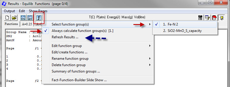
to access the Function-Builder Menu.

      In the menu

      • Select the function group '1. Fe-N2'

      • Check 'Always calculate function groups'

      • Click on 'Refresh Results ...' to refresh the Results Window

      In this example nitrogen gas is equilibrated with Fe(liq) at 1600 C. In page 1 we see p(N2) = 0.29904 atm and %N = 0.025619. The calculated functions are posted at the top of each results page. There are 2 calculated functions, f1 and f2 :
      where f1 = %N / p(N2)1/2 = 0.468..e-01; and f2 = log10(f1) = -1.3293

      For complete details consult the Fact-Function-Builder Slide Show.

  • Phase Diagram
    • Enhanced detailed point calculation

      After a diagram has been displayed, you calculate the equilibrium at any position on the diagram by selecting the 'phase equilibrium mode', and then pointing and clicking at the desired spot.


      In FactSage 7.0, after clicking you now have the option to enter the precise coordinates for the detailed point calculation.


      The screenshot shows the calculated equilibrium in the Cu-O binary system at 1300oC and XO = 0.35 using data from the public FScopp database.

    • Isobars and iso-activity lines - new option 'Z'

      In FactSage 7.0 you can plot isobars of a gas species or gas phase and iso-activity lines of a compound (liquid, solid).

      For a compound species the isobar or iso-activity is defined in the Selection Window (activated in the Menu Window by a mouse-right-click on a 'Compound species' check box). In the Selection Window mouse-right-click on the selected species, select 'Z isobars..' and then enter the values.

      The screenshots show the calculation of O2(g) isobars in the Cu-O binary systems using data from the public FScopp database.

      Left: calculation of O2(g) isobars in the FeO-Fe2O3-Cr2O3 ternary system at 1300oC using data from the public FToxid database.
      Right: calculation of C(s) iso-activity lines in the Fe-Cr-C ternary system using data from the public SGTE2011 database.

      Left: calculation of CaF2(s) iso-activities in CaF2-NaCl-CaCl2-NaF reciprocal salt system at 1000 K using data from the public FTsalt database.
      Right: calculation of C(s) iso-activities in Fe-Cr-C-N paraequilibrium diagram with diffusing elements N and C using data from the public SGTE2011 database.

      Approximately 60 example diagrams with various X- and Y-axes are stored in Phase Diagram. To load and calculate the phase diagrams with isobars and iso-activity lines that are shown above run Phase Diagram and click on 'File > Directories > Phase diagrams with various......'. This list of examples is by no means exhaustive.

  • Viscosity

      The Viscosity module now runs on a server.

      The database for the slag viscosity module has been updated to include more data for systems with fluorides and to improve the data for systems with FeO and Fe2O3.

    3. Databases:


    Previous FactSage Updates

    The following displays are only available if you have updated your installation with that particular version.

    What's New in:


    [F*A*C*T] [www.factsage.com] [GTT]